Tutorial 2 — Grow your first network

Goal: a sensor sheet that projects topographically onto a map, grown from a genome; then stimulate it and check, in this simulation, that neighbouring sensors drive neighbouring map neurons.

1. The body plan

import numpy as np
from neurogenesis.development import BodyPlan, FixedPlacement, Region, grow, region_of

side = 6
sheet = [[(i + 0.5) / side, (j + 0.5) / side, 0.5] for i in range(side) for j in range(side)]

plan = BodyPlan(
    name="topographic map",
    regions=[
        Region("sensor", origin=(0, 0, 0), size=(30, 30, 5), placement=FixedPlacement(sheet), role=1),  # role 1 = input
        Region("map", origin=(50, 0, 0), size=(30, 30, 10)),                                          # grown placement
    ],
    projections=[("sensor", "map")],
)

• A region is a box (origin, size in space units). Positions inside it are local coordinates in [0, 1]³.

• FixedPlacement puts cells at given local positions (supervised); without it, the genome decides how many cells there are and where they migrate.

• Distances in space units set conduction delays (conduction_velocity, default 20 units per tick).

2. The genome

genome = dict(
    count=dict(map=200),                                              # number of map cells
    inh_weight_factor=2.0, w_clip=2047,
    migration=dict(map=dict(mean=np.full(3, 0.5), spread=0.35)),     # where map cells settle
    inhibitory=dict(map=dict(a0=-6.0, a=np.zeros(3))),                # logistic P(inhibitory | position): ~0 here
    guidance={("sensor", "map"): dict(
        B=np.diag([2.0, 2.0, 0.0]), c=np.zeros(3),                    # target position = B @ source position + c
        sigma=0.12, p0=0.9, w=900.0)},                                # tuning width, peak probability, weight
)

Axon guidance is chemoaffinity in its simplest form: each source cell aims at a target position, an affine function of its own position, and connects to cells near that target with a Gaussian probability (width sigma).

3. Grow

net = grow(plan, genome, seed=0)
print(net.num_neurons, net.num_synapses)
sensor, mp = region_of(net, plan, "sensor"), region_of(net, plan, "map")

grow is deterministic: the same seed gives the same network, bit for bit. Different seeds give different individuals of the same “species” (genome).

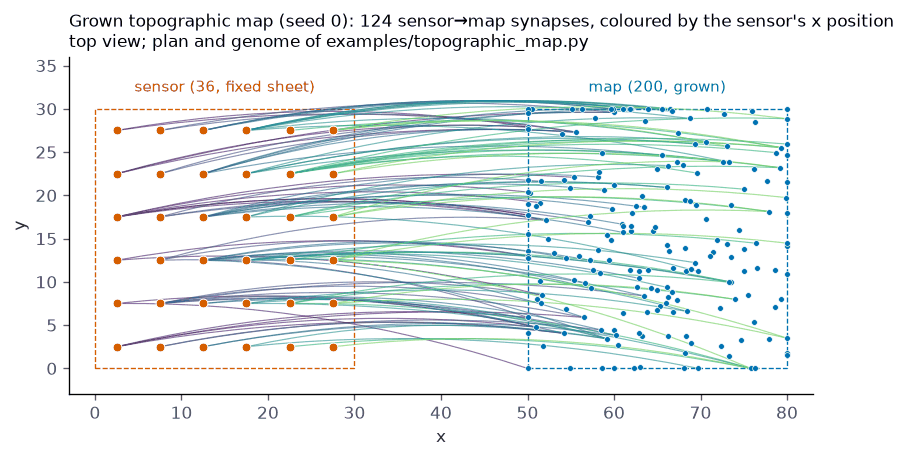
The grown network (seed 0, top view): 36 sensor cells on a fixed sheet (left), 200 map cells placed by the genome (right), and the 124 sensor → map synapses coloured by the sensor’s x position.

4. Stimulate and read out

from neurogenesis.spiking.batch import simulate_counts

ext = np.zeros((2, net.num_neurons), np.int32)    # 2 stimuli × neurons: constant input current
ext[0, sensor[0]] = 120                            # stimulus 1: corner (0, 0) of the sheet
ext[1, sensor[-1]] = 120                           # stimulus 2: corner (1, 1)
counts = simulate_counts([net], [ext], ticks=50, blank=40)[0]   # spike counts per stimulus and neuron

u = np.asarray([(net.neurons[i].x - 50) / 30 for i in mp])      # map position along x, 0..1
for k in range(2):
    c = counts[k, mp]
    print(k, int((c > 0).sum()), (u * c).sum() / c.sum())

simulate_counts runs many networks and many stimuli in one batched JAX call. blank silent ticks precede every stimulus so that responses do not carry over.

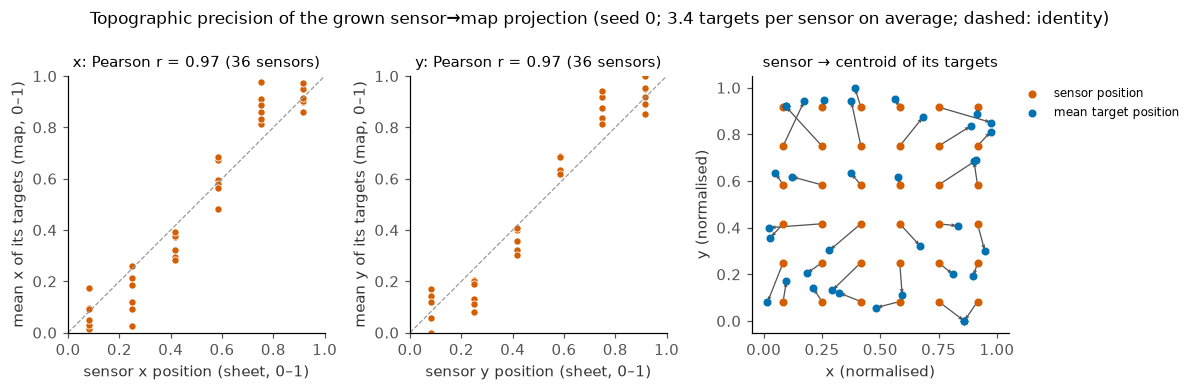
Topography of the grown projection (seed 0): for each of the 36 sensors, its position on the sheet against the mean position of its targets in the map (Pearson r = 0.97 on both axes in this network).

5. Save

net.save_json("network.json")          # for the viewer
from neurogenesis.modules import Module
Module("topographic map", plan, genome, inputs=["sensor"], outputs=["map"],
       description="sensor sheet -> topographic map").save("module.json")

Exercises

1. Increase sigma to 0.3: how does the precision of the map change?

2. Flip the sign of B[0, 0]: which side of the map now responds to stimulus 1?

3. Knock out the projection: from neurogenesis.development import knockout, grow(plan, knockout(genome, projections=[("sensor", "map")]), seed=0).