Tutorial 1 — The command line

The toolbox has two command-line entry points:

Entry point	Purpose
python -m neurogenesis <command> (also installed as neurogenesis)	generate, simulate, inspect networks; estimate costs
python -m neurogenesis.bridge	a JSON server on stdin / stdout used by the desktop apps and by other programs

python -m neurogenesis --help

generate — a network from a preset morphology

python -m neurogenesis generate --neurons 500 --morphology column --weight-scale 0.2 --refractory 3 --out column.json

Generating SNN population (500 neurons, morphology: 'column')...
✓ Network successfully saved to /.../column.json
  Neurons: 500 | Synapses: 7,162

Option	Default	Meaning
--neurons	1000	number of neurons
--morphology	column	column, layered or microcircuit
--exc-ratio	0.80	fraction of excitatory neurons
--pace-ratio	0.05	fraction of driver (pacemaker) neurons
--radius, --height	30, 150	column size (space units)
--layers	4	number of layers (layered)
--conduction-velocity	4.0	space units per tick; sets axonal delays
--weight-scale, --inh-scale	1.0, 1.0	scale all weights / inhibitory weights (column)
--refractory	0	absolute refractory period in ticks (column)
--seed	42	random seed
--out	network.json	output file

These presets are fixed generators, useful for testing the kernels and viewers. Circuits grown from genomes are made in Python (tutorial 2).

simulate — run the integer kernel

python -m neurogenesis simulate --network column.json --ticks 1000 --raster raster.png

Loading network from column.json...
Simulating 500 neurons for 1000 ticks (seed=12345)...
✓ Simulation Complete:
  Total spikes emitted: 11,554
  Mean population rate: 23.11 Hz

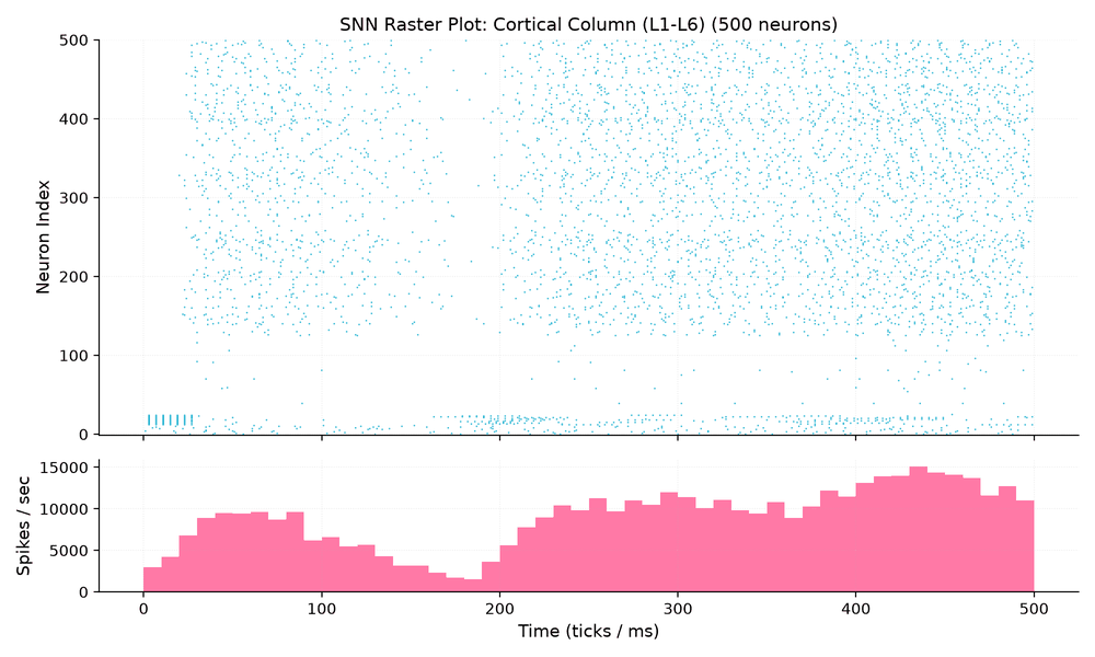
raster.png as written by the command.

stats — topology of a network

python -m neurogenesis stats --network column.json

--- SNN Topology & Biophysical Statistics: Cortical Column (L1-L6) ---
{
  "num_neurons": 500,
  "num_synapses": 7162,
  "density": 0.0287,
  "cell_types": {"excitatory_lif": 375, "inhibitory_lif": 100, "autonomous_burster": 13, "poisson_driver": 12},
  "in_degree": {"mean": 14.32, "std": 7.34, "min": 1, "max": 37},
  ...
}

export-presets — example networks for the viewer

python -m neurogenesis export-presets --out-dir presets/

Writes cortical_column_1000.json, microcircuit_100.json and layered_sheets_600.json.

estimate — memory and time before running

python -m neurogenesis estimate --neurons 3e8 --synapses-per-neuron 5000 --seconds 1
python -m neurogenesis estimate --neurons 1e5 --synapses-per-neuron 1000 --model lif_int --model hh

The first call per model and device runs three short benchmarks and caches the throughput in ~/.cache/neurogenesis/throughput.json. Every batched simulation calls the same estimator and refuses networks that cannot fit (CostError), so you learn that a model is out of reach before trying it.

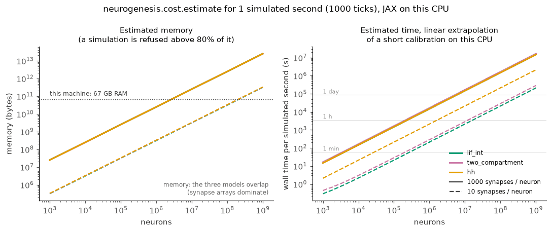
neurogenesis.cost.estimate for one simulated second on the documentation build machine (a 67 GB CPU node), for 10 and 1000 synapses per neuron. Memory is dominated by synapses, so the three models overlap; times are linear extrapolations of a short calibration.

The bridge — the toolbox as a JSON server

python -m neurogenesis.bridge

The server prints a ready event, then answers one JSON request per line:

printf '%s\n' '{"id": 1, "method": "ping"}' \
              '{"id": 2, "method": "estimate", "params": {"neurons": 10000, "synapses": 1000000, "ticks": 1000}}' \
  | python -m neurogenesis.bridge 2>/dev/null

{"event": "ready", "data": {"python": "3.11.15", "protocol": "1.0", "ngb": 1}}
{"id": 1, "result": "pong"}
{"id": 2, "result": {"estimates": [{"model": "lif_int", "neurons": 10000, "synapses": 1000000, "ticks": 1000,
  "memory_bytes": 25640000, "fits": true, "seconds_total": 15.48, "verdict": "fits (memory 25.6 MB of 66.8 GB available); ...

Any program that can start a process and read lines can drive development, simulation, evolution and modules this way. See Driving the toolbox from other programs (the bridge) and the full Bridge protocol, version 1.0.

PLACEHOLDER

Planned commands: neurogenesis run project.json (run a Project’s schedule and save the network), neurogenesis stages --json and neurogenesis ui-schema (catalogue of stages and Params, task H3), neurogenesis validate module.json (re-run a module’s assays, task E4), neurogenesis data fetch (connectome datasets, task I1). An animated terminal recording (asciinema) of this tutorial.